This is the third and final part of decision tree tutorial. In last two parts we talked about introduction to decision tree, impurity measures and CART algorithm for generating the tree.
Here is the part 1 part 2
In this tutorial we will learn about iterative dichotomiser 3 (ID3).
ID3 uses entropy as metric and it is used for classification problem
So, lets start.
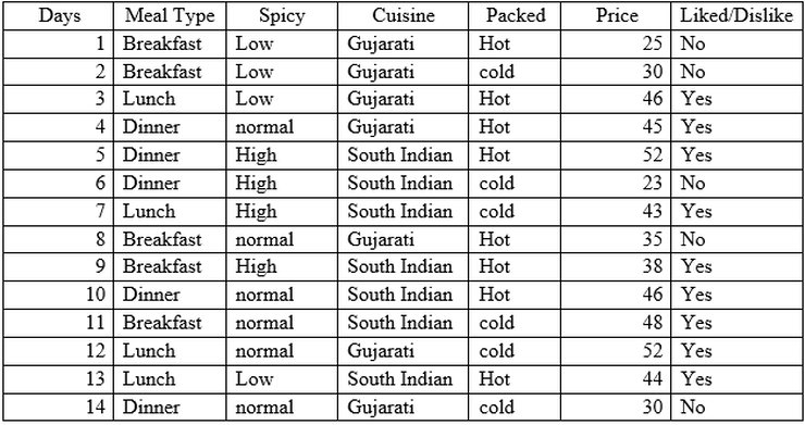
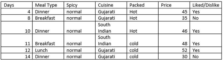
Here we will take the same data set, that we have taken earlier, where the target variable is whether customer liked food or not and predictors are Meal type, Spicy, Cuisine and packed.
Formula for building ID3 tree is:
Let us find entropy of target variable.
From above dataset we have
- Number of observations = 14
- Number of observations having Decision ‘Yes’ = 9
- probability of ‘Yes’, p(Yes) = 9/14
- Number of observations having Decision ‘No’ =5
- probability of ‘No’, p(No) = 5/14
Now let’s find information gain on Meal type .
Number of instances for Meal type = Breakfast is 5
Number of instances for Meal type = Breakfast is 5
Decision =’Yes’, prob (Liked/Dislike=’Yes’ | Meal type = Breakfast) =2/5
Decision =’No’, prob (Liked/Dislike =’No’ | Meal type = Breakfast) =3/5
Entropy (Liked/Dislike | Meal type = Breakfast) = -(2/5) *log2(2/5) – (3/5) * log2(3/5) = 0.97
Number of instances for Meal type = Dinner is 5
Number of instances for Meal type = Dinner is 5
Decision =’Yes’, prob (Liked/Dislike=’Yes’ | Meal type = Dinner) =3/5
Decision =’No’, prob (Liked/Dislike =’No’ | Meal type = Dinner) =2/5
Entropy (Liked/Dislike | Meal type = Dinner) = -(2/5) *log2(2/5) – (3/5) * log2(3/5) = 0.97
Number of instances for Meal type = Lunch is 4
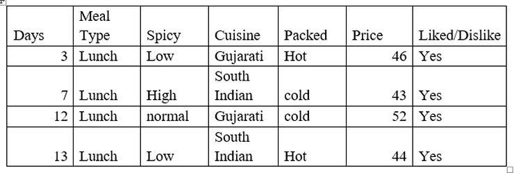
Decision =’Yes’, prob (Liked/Dislike=’Yes’ | Meal type = Dinner) =2/4
Decision =’No’, prob (Liked/Dislike =’No’ | Meal type = Dinner) =2/4
Entropy (Liked/Dislike | Meal type = Lunch) = -(4/4) *log2(4/4) = 0
Gain (Liked/Dislike | Meal type) = Entropy (Liked/Dislike) – p(Liked/Dislike | Meal type = Breakfast)
* log2 p(Liked/Dislike | Meal type = Breakfast) – p(Liked/Dislike | Meal type = Dinner) * log2 p(Liked/Dislike | Meal type = Dinner) – p(Liked/Dislike | Meal type = Lunch) * log2 p(Liked/Dislike | Meal type = Lunch)
Gain (Liked/Dislike | Meal type) = 0.94 – (5/14) * 0.97 – (5/14) * 0.97 – (4/4) *0 = 0.247
Now let’s find information gain Spicy
Number of instances for spicy = high is 4.
Decision =’Yes’, prob (Liked/Dislike=’Yes’ | spicy = high) =3/4
Decision =’No’, prob (Liked/Dislike =’No’ | spicy = high) =1/4
Entropy (Liked/Dislike | spicy = high) = -(3/4) *log2(3/4) – (1/4) * log2(1/4) = 0.81
Number of instances for spicy = Low is 4.
Decision =’Yes’, prob (Liked/Dislike=’Yes’ | spicy = Low) =2/4
Decision =’No’, prob (Liked/Dislike =’No’ | spicy = Low) =2/4
Entropy (Liked/Dislike | spicy = Low) = -(3/4) *log2(3/4) – (1/4) * log2(1/4) = 1
Number of instances for spicy = Normal is 6.
Decision =’Yes’, prob (Liked/Dislike=’Yes’ | spicy = Normal) =4/6
Decision =’No’, prob (Liked/Dislike =’No’ | spicy = Normal) =2/6
Entropy (Liked/Dislike | spicy = Normal) = -(4/6) *log2(4/6) – (2/6) * log2(2/6) = 0.92
Gain (Liked/Dislike | Spicy) = 0.94 – (4/14) * 0.81 – (4/14) * 1 – (6/14) *0 .92= 0.028
Similarly, we will calculate Gain value for Cuisine and packed
Gain (Liked/Dislike | Cuisine) = 0.94- ((7/14) *0.98) -((7/14) *0.59) = 0.155
Gain (Liked/Dislike | Packed) = 0.94- ((8/14) *0.81) -((6/14) *1) = 0.048
Summary of information gain for all attributes is:
- Gain (Liked/Dislike | Meal type) = 0.247
- Gain (Liked/Dislike | Spicy) = 0.028
- Gain (Liked/Dislike | Cuisine) = 0.155
- Gain (Liked/Dislike | Packed) = 0.048
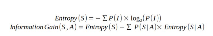
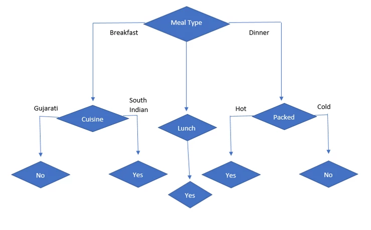
As we can see that Meal type has highest information gain, our first node is Meal Type.
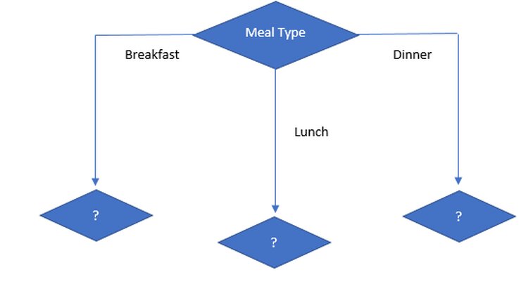
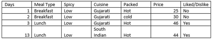
Information gain on meal type under breakfast is:
Entropy (Liked/Dislike | Meal Type = Breakfast) = = -(2/5) *log2(2/5) – (3/5) * log2(3/5) = 0.97
Entropy (Breakfast | Spicy = Low) = -(0/2) *log2(0/2) – (2/2) * log2(2/2) = 0
Entropy (Breakfast | Spicy = Normal) = -(1/2) *log2(1/2) – (1/2) * log2(1/2) = 1
Entropy (Breakfast | Spicy = High) = -(1/1) *log2(1/1) – (0/1) * log2(0/1) = 0
Gain (Breakfast,Spicy) = 0.57
Entropy (Breakfast | Cuisine = Gujarati) = -(0/3) *log2(0/3) – (3/3) * log2(3/3) = 0
Entropy (Breakfast | Cuisine = South Indian) = -(2/2) *log2(2/2) – (0/2) * log2(0/2) = 0
Gain (Breakfast,Cuisine) = 0.97
Entropy (Breakfast | Packed = Hot) = -(2/3) *log2(2/3) – (1/3) * log2(1/3) = 0.9183
Entropy (Breakfast | Packed = Cold) = -(1/2) *log2(1/2) – (1/2) * log2(1/2) = 1
Gain (Breakfast,Cuisine) = 0.97- ((3/5) *0.92) -((2/5) *1) = 0.018
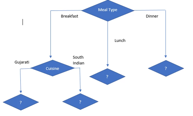
As we can see cuisine is higher attribute than any other, so our next node is cuisine.
Information gain on Meal type = Lunch
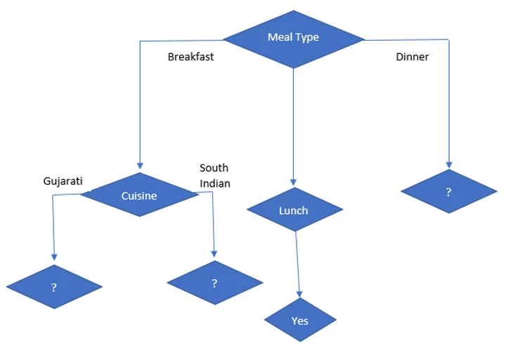
As we can see all observations say “Yes”,
So, entropy (Liked/Dislike | Lunch) = 0
So, if Meal type = Lunch then it is “Yes” and it is leaf node. So no further division is possible.
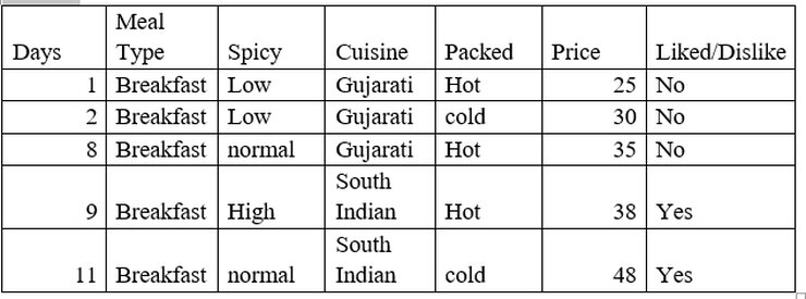
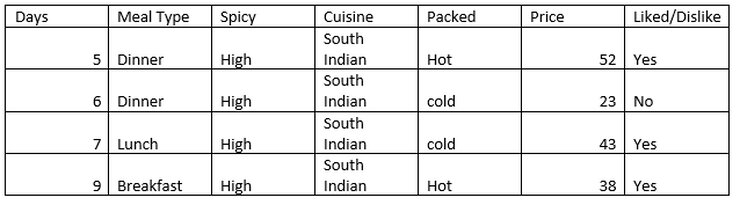
Information gain on Meal type = Dinner
Number of instances for Meal type = Dinner is 5
Decision =’Yes’, prob (Liked/Dislike=’Yes’ | Meal type = Dinner) =3/5
Decision =’No’, prob (Liked/Dislike =’No’ | Meal type = Dinner) =2/5
Entropy (Liked/Dislike | Meal type = Dinner) = -(2/5) *log2(2/5) – (3/5) * log2(3/5) = 0.97
Gain (Dinner | Spicy) = 0.019
Gain (Dinner | Packed) = 0.97
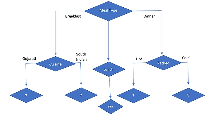
So, packed attribute has highest information gain. so, it is selected as next node under dinner.
Now, we will select Meal Type = Breakfast and Cuisine

So, when cuisine = Gujarati, we can see that decision is always No and when cuisine = South Indian, we can see that decision is always Yes.
Now, we will select Meal Type = Dinner and Packed
So, when packed = Hot, we can see decision is always Yes and when Packed = cold, we can see that decision is always No.
So final decision tree is.
Happy Learning 🙂

 5
5
Leave a comment