As we have seen how to generate classification decision tree using Gini index/Gini impurity in Part I.
Here is the link : Part I
Now let’s move to create Regression decision tree using CART.
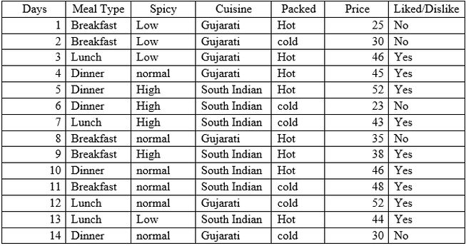
We are going to take same example but the target variable is “Price”.
Standard Deviation reduction
We are going to construct decision tree that involves partitioning data into subsets that contains instances with similar values (homogeneous). We will use standard deviation to calculate homogeneity. If the numerical sample is completely homogeneous its standard deviation is zero.
Standard deviation reduction is standard deviation of target variable subtracted from standard deviation of predictors, so higher standard deviation reduction means more homogeneity in data that will help to identify predictor variable for splits.
Here we will use 3 statistics to generate decision tree.
1. Standard deviation (S) is for tree building (branching)
2. Coefficient of variation (CV) is used to decide when to stop branching. We can use Count (n) as well.
3. Average (Avg) is the value in the leaf nodes.
Thus, for price attribute,
- Count = n = 14
- Average = 39.8
- Standard deviation = 9.32
- Coefficient of variation (CV) = 23%
Now let us find standard deviation reduction for target and predictors.
Standard deviation for two variables:
Meal Type
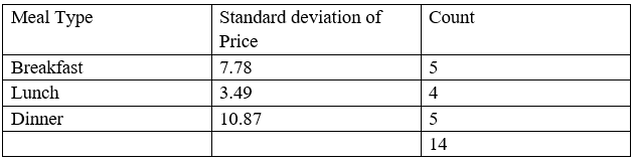
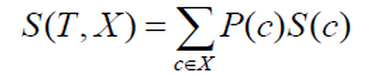
Standard deviation (Meal Type) = P(Breakfast) * S(Breakfast) + P(Lunch) * S (Lunch) + P (Dinner) * S(Dinner)
= (5/14) *7.78 + (4/14) * 3.49 + (5/14) *10.87
= 2.78 + 0.99 + 3.88
= 7.66
Standard deviation reduction for meal type = standard deviation of price– standard deviation of meal type
= 9.32 – 7.66
= 1.66
Spicy
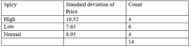
Standard deviation (Spicy) = P(High) * S(High) + P(Low) * S (Low) + P (Normal) * S(Normal)
= (4/14) *10.52 + (6/14) * 7.65 + (4/14) *8.95
= 3.003 + 3.28 + 2.56
= 8.84
Standard deviation reduction for spicy = standard deviation of price – standard deviation of spicy
= 9.32 – 8.84
= 0.48
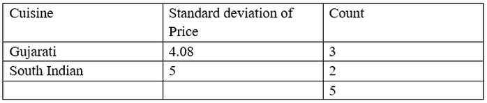
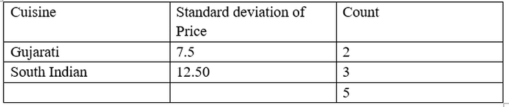
Cuisine
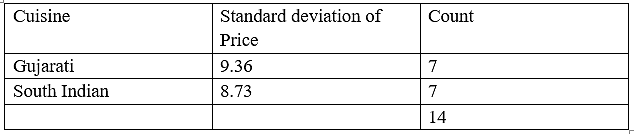
Standard deviation (Cuisine) = P(Gujarati) * S(Gujarati) + P (South Indian) * S (South Indian)
= (7/14) *9.36+ (7/14) * 8.73
= 4.68 + 4.37
= 9.048
Standard deviation reduction for spicy = standard deviation of price – standard deviation of spicy
= 9.32 – 9.048
= 0.272
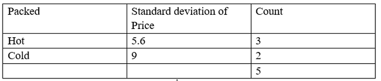
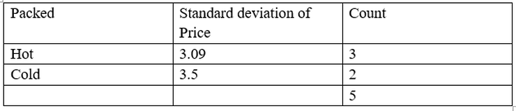
Packed
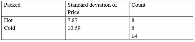
Standard deviation (Packed) = P(Hot) * S(Hot) + P (Cold) * S (Cold)
= (8/14) *7.87+ (6/14) * 10.59
= 4.49 + 4.54
= 9.04
Standard deviation reduction for spicy = standard deviation of price – standard deviation of spicy
= 9.32 – 9.048
= 0.27
So standard deviation reduction for all predictors are as follows:
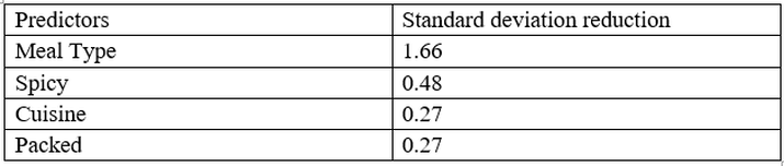
The attribute with the largest standard deviation reduction is chosen for the decision node, so our first split is Meal Type.
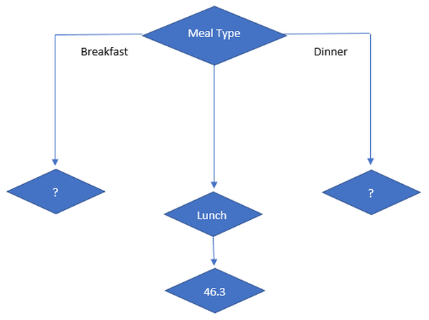
So, our initial decision tree looks like
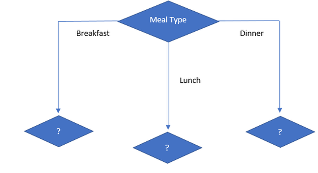
Now we will decide next split on basis of coefficient of variation (CV).
The coefficient of variation (CV) is a measure of relative variability. It is the ratio of the standard deviation to the mean (average). So here “The standard deviation is 23% of the mean” is a CV. So, The higher the coefficient of variation, the greater the level of dispersion around the mean. The lower the value of the coefficient of variation, the more precise the estimate that is more homogeneity.
So, here we know CV = 23% so we can set threshold < 23%. Let’s say 10% is threshold for CV.
So, Let’s have CV for Meal Type
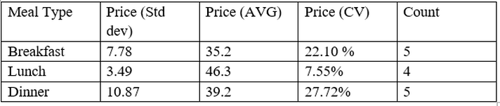
Lunch don’t need any further splitting as its CV is 8% which is less than 10%(threshold)
Thus, decision tree looks like:
Now, we have to decide split on breakfast and dinner as CV is > 10% for both.
So, our sub data looks like:
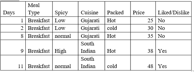
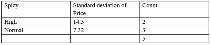
So, when meal type = breakfast then
- Std dev = 7.78
- Avg = 35.2
- Count = 5
- CV = 22%
So, when meal type = breakfast then second decision node is:
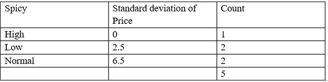
- Standard Deviation Reduction (spicy) = 7.78 – 3.6 = 4.42
- Standard Deviation Reduction (Cuisine) = 7.78 – 4.45 = 3.33
- Standard Deviation Reduction (Packed) = 7.78 – 6.9346664 = 0.84
So, the next best node is spicy. so, decision tree looks like
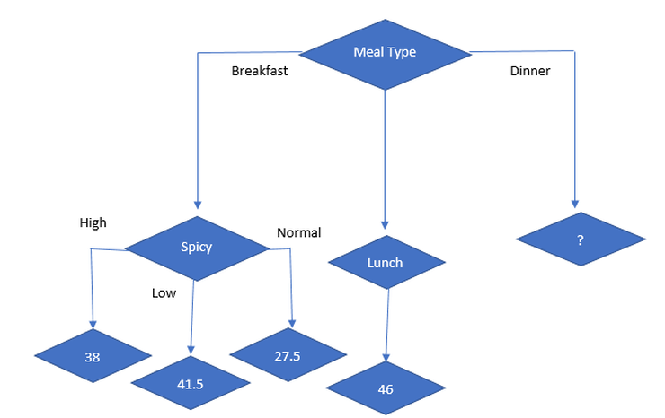
Now, lets start with split on dinner.
So, our sub data looks like:
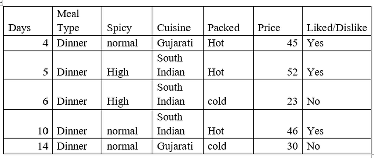
So, when meal type = dinner then
- Std dev = 10.87
- Avg = 39.2
- Count = 5
- CV = 28%
- Standard Deviation Reduction (spicy) = 10.87 – 10.19 = 0.68
- Standard Deviation Reduction (cuisine) = 10.87 – 10.49 = 0.37
- Standard Deviation Reduction (packed) = 10.87 – 3.25 = 7.62
So highest standard deviation reduction is packed, so final decision tree looks like.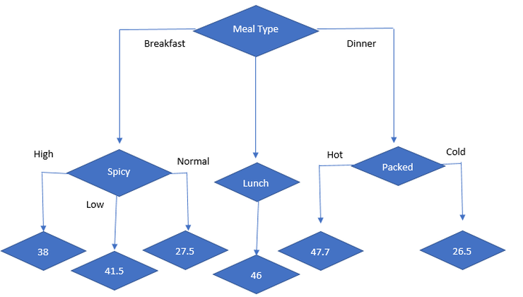
We will continue with the ID3 tree in the next article.
Happy Learning.

 23
23