Introduction
From classrooms to corporate, one of the first lessons in machine learning involves decision trees. Mathematics behind decision tree is very easy to understand compared to other machine learning algorithms. Decision tree is also easy to interpret and understand compared to other ML algorithms.
If you are just getting started with machine learning, it’s very easy to pick up decision trees. In this tutorial, you’ll learn:
1. What is a decision tree?
2. Algorithms used in constructing a decision tree
- Gini index / Gini impurity
- Entropy
- Information gain
- Standard Deviation Reduction
3. Decision tree types
- Classification and regression tree – CART
- ID 3
What is a decision tree?
Decision tree is a supervised learning algorithm that works for both categorical and continuous input and output variables that is we can predict both categorical variables (classification tree) and a continuous variable (regression tree).
Its graphical representation makes human interpretation easy and helps in decision making.
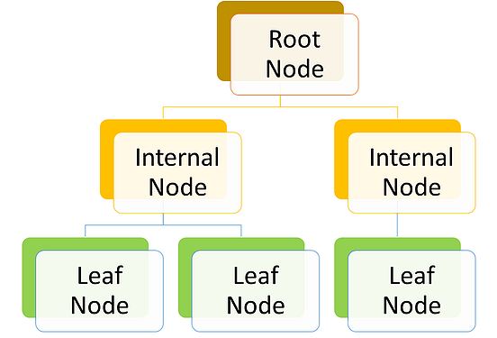
Decision tree is a flow chart like structure with the if-else condition. The top node is the root node, you start question from root node then move through the tree branches according to which groups you belong to until you reach a leaf node.
This article is all about understanding the full mathematical concept of the decision tree algorithm. So, let’s start.
Algorithms used in constructing decision tree
For understanding decision tree algorithm better, let us first understand “impurity” and types of measures of impurity.
What is impurity?
Let us understand impurity from the below image.
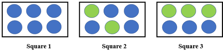
So, there are two round objects of blue and green color inside a square and there are 3 squares. So now how much information I need in each square to accurately identify the color of round objects. So, square 1 needs less information as all objects are blue, square 2 needs little more information than square 1 to tell accurately the color of the object and square 3 requires maximum information as both blue and green objects are equal in number.
As information is a measure of purity, square 1 is a pure node, square 2 is less impure and square 3 is more impure.
So how to measure impurity in data?
In this article, we are going to look at two such impurity measure
- Entropy
- Gini index/ Gini impurity
- Standard deviation
Entropy
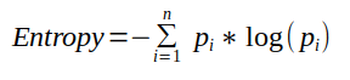
Entropy is the amount of information needed to accurately describe data. So, if data is homogenous that is all elements are similar then entropy is 0 (that is pure), else if elements are equally divided then entropy move towards 1 (that is impure).
So, square 1 has the lowest entropy, square 2 has more entropy and square 3 has the highest entropy.
Mathematically it is written as:
Gini index/Gini impurity
It measures impurity in the node. It has a value between 0 and 1. So the Gini index of value 0 means sample are perfectly homogeneous and all elements are similar, whereas, Gini index of value 1 means maximal inequality among elements. It is sum of the square of the probabilities of each class. It is illustrated as,

So, (Im)purity measures homogeneity in data and if data is homogenous then it belongs to the same class and decision tree splits on homogeneity.
Decision tree types
There are various algorithm that used to generate decision tree, some are as following
- ID3 (Iterative Dichotomiser 3)
- ID 4.5 (successor of ID3)
- CART (Classification and Regression Tree)
- CHAID (Chi-squared Automatic Interaction Detector)
- In this article, we will talk about CART and ID3 that are mostly used in the industry.
CART
It is used for both classification and regression. Let us understand classification (CA) and regression tree (RT)
- Classification tree
- A decision tree where target variable is categorical
- The algorithm classifies the class within which the target variable would most likely to fall
- It uses Gini index as metric/cost function to evaluate split in feature selection
- Example like predicting who will or who will not order food, whether the weather will be rainy, sunny or cool
2. Regression tree
- A decision tree where the target variable is continuous/discrete
- Algorithm predicts value
- It uses least square / standard deviation reduction as a metric to select features in case of the Regression tree.
- Example like predicting the price of a house, predicting the sell of crops
Let’s start with the classification tree.
Let’s start with a dataset that is hypothetical, where the target variable is whether the customer liked the food or not.
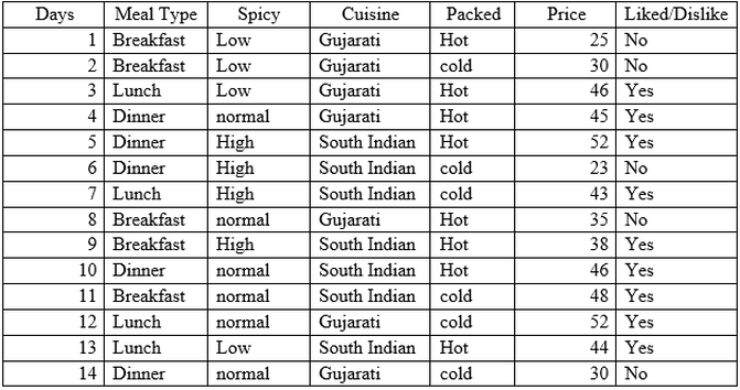
From the above data, Meal type, Spicy, Cuisine and packed are the inputs/features of data and liked/dislike is the target variable.
Now let’s start building tree having Gini index as im(purity) measure.
Meal Type
Meal Type is a nominal data that has 3 values Breakfast, Lunch and Dinner. Let’s classify the instances on basis of liked/dislike.
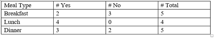
Gini index (Meal Type = Breakfast) = 1-(2/5) ²+(3/5) ² = 1- (0.16+0.36) = 0.48
Gini index (Meal Type = Lunch) = 1- (4/4) ²+(0/4) ² = 1- (1+ 0) = 0
Gini index (Meal Type = Dinner) = 1- (3/5) ² +(2/5) ² = 1- (0.36+0.16) = 0.48
Now, we will calculate the weighted sum of Gini index for Meal Type features,
Gini (Meal Type) = (5/14) *0.48 + (4/14) *0 + (5/14) *0.48 = 0.342
Spicy
Spicy is a nominal data that has 3 values Low, Normal and High. Let’s classify the instances on basis of liked/dislike.
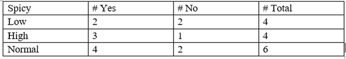
Gini (Spicy = Low) = 1-(2/4) ²+(2/4) ² = 0.5
Gini (Spicy = High) = 1-(3/4) ²+(1/4) ² = 0.375
Gini (Spicy = Normal) = 1-(4/6) ²+(2/6) ² = 0.445
Now, the weighted sum of Gini index for Spicy features can be calculated as,
Gini (Spicy)= (4/14) *0.5 + (4/14) *0.375 + (6/14) *0.445 =0.439
Cuisine
The cuisine is a binary data that has 2 values Gujarati and south Indian. Let’s classify the instances on the basis of liked/dislike.
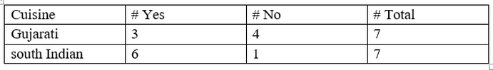
Gini (Cuisine = Gujarati) = 1-(3/7) ²+(4/7) ² = 0.489
Gini (Cuisine =south Indian) = 1-(6/7) ²+(1/7) ² = 0.244
Now, the weighted sum of the Gini index for Cuisine features can be calculated as,
Gini (Cuisine) = (7/14) *0.489 + (7/14) *0.244=0.367
Packed
Packed is a binary data that has 2 values Hot and cold. Let’s classify the instances on the basis of liked/dislike.
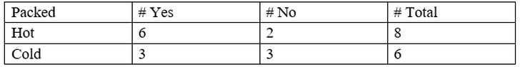
Gini (Packed = Hot) = 1-(6/8) ²+(2/8) ² = 0.375
Gini (Packed = Cold) = 1-(3/6) ²+(3/6) ²= 0.5
Now, the weighted sum of the Gini index for Packed features can be calculated as,
Gini (Packed) = (8/14) *0.375 + (6/14) *0.5=0.428
So, the Gini index for all the feature is:
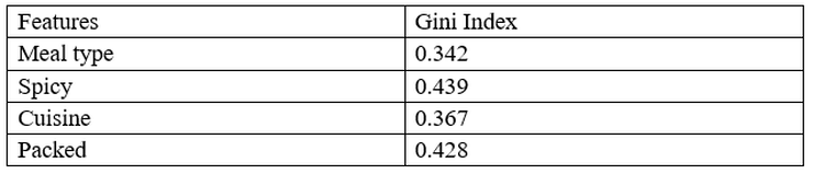
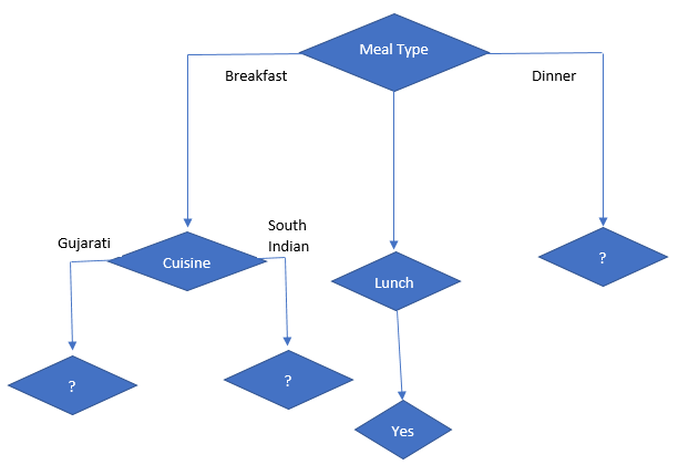
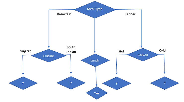
So, we can conclude that the lowest Gini index is of “Meal Type” and a lower Gini index means the highest purity and more homogeneity. So, our root node is “Meal type”. So, our tree looks like
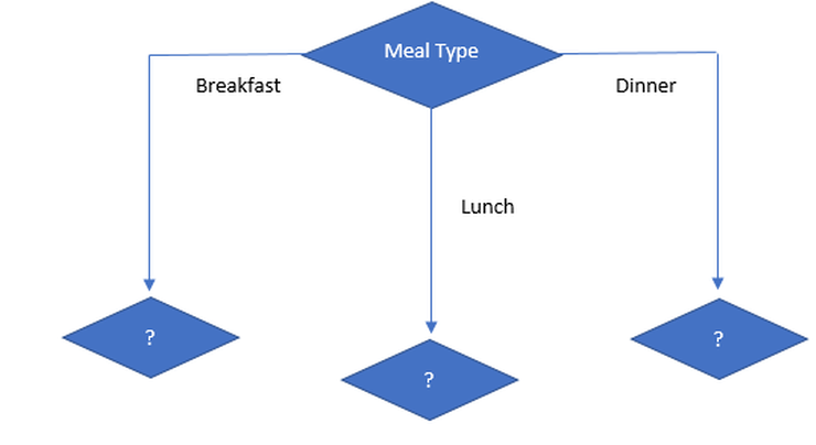
Let’s calculate the next split with the Gini index on the sub data set for the Meal Type feature, we will use the same method as above to find the next split.
Let’s find the Gini index of spicy, cuisine and packed on sub-data of Meal type = Breakfast.
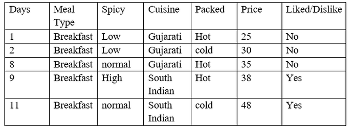
Gini index for Spicy on breakfast meal type
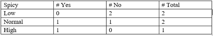
Gini (Meal type = Breakfast & Spicy = Low) = 1-(0/2) ²+(2/2) ² = 0
Gini (Meal type = Breakfast & Spicy = High) = 1-(1/1) ²+(0/1) ² = 0
Gini (Meal type = Breakfast & Spicy = Normal) = 1-(1/2) ²+(1/2) ² = 0.5
Now, the weighted sum of Gini index for temperature on sunny outlook features can be calculated as,
Gini (Meal type = Breakfast & Spicy) = (2/5) *0 + (1/5) *0+ (2/5) *0.5 =0.2
Gini index for cuisine on breakfast meal type
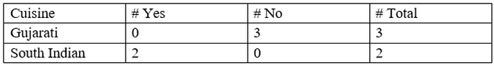
Gini (Meal type = Breakfast & Cuisine = Gujarati) = 1-(0/3) ²+(3/3) ² = 0
Gini (Meal type = Breakfast & Cuisine = South Indian) = 1-(2/2) ²+(0/2) ² = 0
Now, the weighted sum of Gini index for humidity on sunny outlook features can be calculated as,
Gini (Meal type = Breakfast & Cuisine) = (3/5) *0 + (2/5) *0=0
Gini index for packed on breakfast meal type
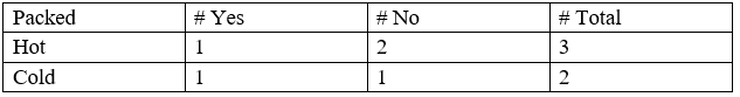
Gini (Meal type = Breakfast & Packed = hot) = 1-(1/3) ²+(2/3) ² = 0.44
Gini (Meal type = Breakfast & Packed = cold) = 1-(1/2) ²+(1/2) ² = 0.5
Now, the weighted sum of Gini index for wind on sunny outlook features can be calculated as,
Gini (Meal type = Breakfast and Packed) = (3/5) *0.44 + (2/5) *0.5=0.266+0.2= 0.466
According to the Gini index, Decision on Breakfast Meal Type is:
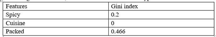
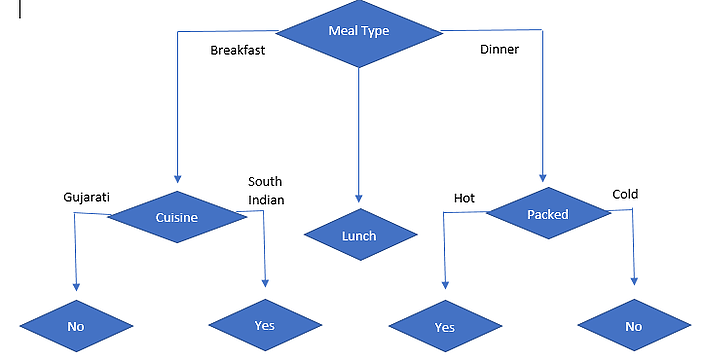
As we can see for the breakfast meal type, the cuisine has the lowest Gini value that is highly homogenous and highest pure amongst other features, so we can conclude that the next node will be cuisine. So, the tree will be like:
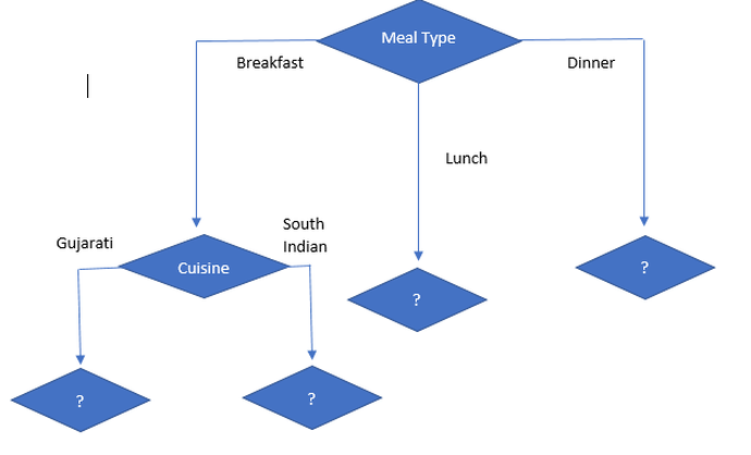
Now let’s focus on sub-data of Meal Type = Lunch
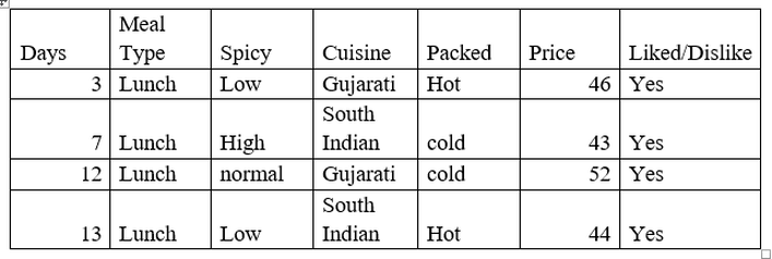
As we can see for Meal Type = Lunch, the target variable is “Yes” for all so the Gini index is 0 that is there is no impurity and it is highly homogenous. So, it’s a leaf node.
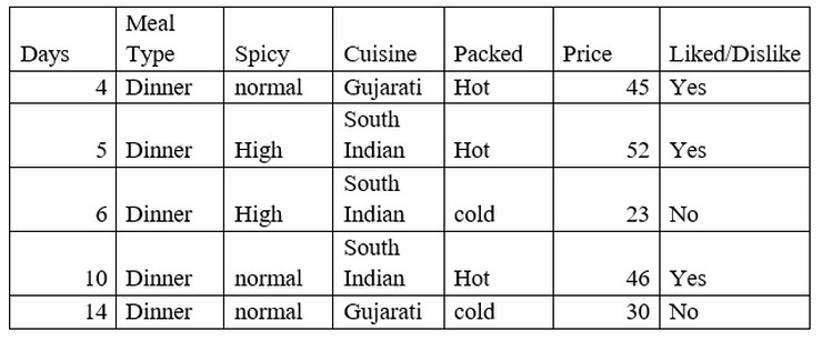
Now, let’s focus on Meal Type = Dinner and find the Gini index for spicy, cuisine and packed.
Gini index for spicy on meal type = Dinner
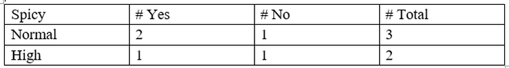
Gini (meal type = Dinner and Spicy= High) = 1 – (1/2)2 + (1/2)2 = 0.5
Gini (meal type = Dinner and Spicy = Normal) = 1 – (2/3)2 + (1/3)2 = 0.444
Gini (meal type = Dinner and Spicy) = (2/5) *0.5 + (3/5) *0.444 = 0.466
Gini index for cuisine on meal type = Dinner
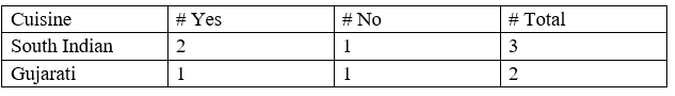
Gini (meal type = Dinner and Cuisine = Gujarati) = 1 – (1/2)2 + (1/2)2 = 0.5
Gini (meal type = Dinner and Cuisine = South Indian) = 1 – (2/3)2 + (1/3)2 = 0.444
Gini (meal type = Dinner and Cuisine) = (2/5) *0.5 + (3/5) *0.444 = 0.466
Gini index for Packed on meal type = Dinner
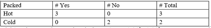
Gini (meal type = Dinner and Packed = Hot) = 1 – (3/3)2 + (0/3)2 = 0
Gini (meal type = Dinner and Packed = Cold) = 1 – (0/2)2 + (2/2)2 = 0
Gini (meal type = Dinner and Packed) = (3/5) *0 + (2/5) *0 = 0
The decision on Meal Type = Dinner
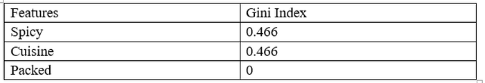
So, packed has the lowest Gini value, so the next node will be packed and the following is a decision tree.
Now, let’s focus on sub-data of:
1. Cuisine
-
Gujarati
-
South Indian
2. Packed
-
Hot
-
Cold
First, we will focus on Meal Type= Breakfast and Gujarati and south Indian cuisine
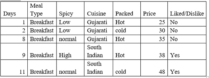
As we can see that when Meal Type = Breakfast and Cuisine = Gujarati then the decision is always No
And when Meal Type = Breakfast and Cuisine = South Indian then the decision is always Yes.
So we got the leaf nodes.
Now we will focus on Meal Type= Dinner and hot and cold packed
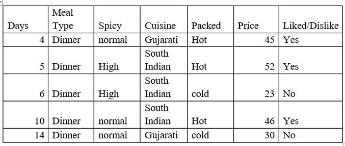
As we can see that when Meal Type = Dinner and Packed = Hot then the decision is always Yes
And when Meal Type = Dinner and Packed = Cold then the decision is always No.
So, we got the leaf nodes.
The following is our final classification decision tree:
We will continue with the regression tree and ID3 tree in the next articles.
Happy Learning.

 63
63
Leave a comment