Introduction to Time Series Forecasting
Time series are everywhere
- Situation 1: You are owning a restaurant and you observe a pattern that highest customers are on weekends
- Situation 2: You are selling a product and you predict raw materials required for that product at a particular moment in the future.
- Situation 3: You are monitoring a data center and you want to detect any anomaly such as abnormal CPU usage which might cause downtime on your servers. You follow the curve of the CPU usage and want to know when an anomaly occurs.
In each of the situations, we are dealing with time series.
Last article we saw various components of time series and forecasting methods using excel and python.
Here is the link to my previous blog : https://www.datascienceprophet.com/time-series-forecasting-i/
Here in this article, we will cover:
- Holt’s Linear smoothing
- Holt’s Damped Trend
Holt’s Linear smoothing
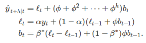
Holt (1957) extended simple exponential smoothing to allow the forecasting of data with a trend. This method involves a forecast equation and two smoothing equations (one for the level and one for the trend). Holt’s Linear Trend Method is also called double Exponential Smoothing.
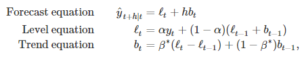
where ℓt denotes an estimate of the level of the series at time t, bt denotes an estimate of the trend (slope) of the time series at time t, α is the smoothing parameter for the level, 0≤α≤1, and β∗ is the smoothing parameter for the trend, 0≤β≤1.
As with simple exponential smooth (SES), the level equation here shows that ℓt is a weighted average of observation yt and the one-step-ahead training forecast for time t, here given by ℓt−1+bt−1. The trend equation shows that bt is the weighted average of the estimated trend at time t based on ℓt−ℓt−1 and bt−1, the previous estimate of the trend.
The forecast function is no longer flat but trending. The h-step-ahead forecast is equal to the last estimated level plus h times the last estimated trend value. Hence the forecasts are a linear function of h.
Holt’s linear smoothing is used when there is a trend in data and there is no seasonality.
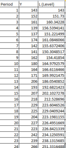
Let us take the below data
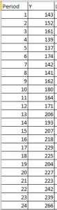
Now, we will calculate the level with the following formula:
![]()
So when y = 152 and alpha = 0.4 and beta = 0.3 then level = 0.4*152 + ( 1 – 0.4)*(143 + 9) = 152 ( Here when y = 143 that is first row the level is same as value of y so it is 143 and slope is y2-y1 that is 152 – 143 = 9 ) , which is $M$2*B4+(1-$M$2)*(C3+D3) in excel book
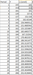
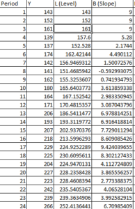
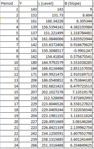
Now we will calculate the trend/slope
![]()
so when y = 152 and alpha = 0.4 and beta = 0.3 then Trend/slope = 0.3*(152-143) + (1-0.3)*9 = 9, so in excel it would be $M$2*B5+(1-$M$2)*(C4+D4)
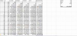
Now we will calculate the forecast, so the following is the equation for the forecast.
![]()
So when y = 139 , level and trend of previous period is added so forecast = 161 + 9 = 170
Next is calculating forecast error , so for y = 139 , error is 139-170 = -31 and squared error is = -31^2 = 669.77 and MSE is the average sum of squared error.
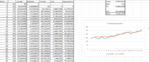
Thus final solution looks like this.
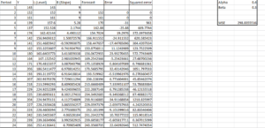
So MSE = 298.83
Now, let us optimize this solution.
We can optimize this solution by minimizing MSE using excel solver by changing alpha and beta values.
So after using excel solver the optimized value is Alpha = 0.5 and Beta = 0.07
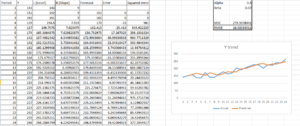
So MSE = 274.91
Thus with excel solver, we decreased squared error and optimized the model with good accuracy.
If you observe the plot, it also shows that actual and predicted values are close to each other.
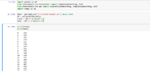
Let us code in python and find prediction when y = 266 when alpha is 0.4 and beta is 0.3 and then when we change alpha to 0.5 and beta to 0.07
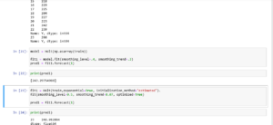
Thus we can see that predictions for y are the same in excel and python both
Now let us use the same data and predict using Holt’s damped trend.
Holt’s Damped trend
The forecasts generated by Holt’s linear method display a constant trend (increasing or decreasing) indefinitely into the future. Empirical evidence indicates that these methods tend to over-forecast, especially for longer forecast horizons. Motivated by this observation, Gardner & McKenzie (1985) introduced a parameter that “dampens” the trend to a flat line sometime in the future. Methods that include a damped trend have proven to be very successful, and are arguably the most popular individual methods when forecasts are required automatically for many series.
In conjunction with the smoothing parameters α and β (with values between 0 and 1 as in Holt’s method), this method also includes a damping parameter 0<ϕ<1:
If ϕ=1, the method is identical to Holt’s linear method. For values between 0 and 1, ϕ dampens the trend so that it approaches a constant some time in the future. In fact, the forecasts converge to ℓT+ϕbT/(1−ϕ) as h→∞ for any value 0<ϕ<1. This means that short-run forecasts are trended while long-run forecasts are constant.
In practice, ϕ is rarely less than 0.8 as the damping has a very strong effect for 14er values. Values of ϕ close to 1 will mean that a damped model is not able to be distinguished from a non-damped model. For these reasons, we usually restrict ϕ to a minimum of 0.8 and a maximum of 0.98.
Now, we will calculate the level with the following formula:
![]()
So when y = 152 and alpha = 0.4 and beta = 0.3 then level = 0.4*152 + ( 1 – 0.4)*(143 + (0.95*9)) = 151.73 ( Here when y = 143 that is first row the level is same as value of y so it is 143 and slope is y2-y1 that is 152 – 143 = 9 ) , which is $M$2*B4+(1-$M$2)*(C3+$M$4*D3) in excel book
Now we will calculate the trend/slope
![]()
so when y = 152 and alpha = 0.4 and beta = 0.3 then Trend/slope = 0.3*(152-143) + (1-0.3)*9 *0.95 = 8.604, so in excel it would be $M$3*(C4-C3)+(1-$M$3)*$M$4*D3
Now we will calculate the forecast, so the following is the equation for the forecast.
![]()
So when y = 139 , level and trend of previous period is added so forecast = 160.34 + 8.30 = 160.334
Next is calculating forecast error , so for y = 139 , error is 139-168.64 = -29.65 and squared error is = -29.64^2 = 878.98 and MSE is the average sum of squared error.
Thus final solution looks like this.
As you can see errors have increased and MSE which was around 274 earlier with a holt linear trend is now 291 with Holt damped trend
Now, let us optimize this solution.
We can optimize this solution by minimizing MSE using excel solver by changing alpha, beta, and phi values.
So after using excel solver the optimized value is Alpha = 0.5 and Beta = 0.01 and phi = 0.965
Thus, MSE is 268.34
Thus damped trend with optimized value is giving us the best prediction result.
Let us code in python and find prediction when y = 266 when alpha is 0.4 ,beta is 0.3 and phi is 0.95 and then when we change alpha to 0.5 ,beta to 0.01 and phi = 0.95
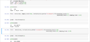
Thus we can see that predictions for y are similar in excel and python both
Hence Holt’s damped trend is showing better forecast with fewer errors and high accuracy in comparison to other trials.
In a review of evidence-based forecasting, Armstrong (2006) recommended the damped trend as a well-established forecasting method that should improve accuracy in practical applications. In a review of forecasting in operational research, Fildes et al. (2008) concluded that the damped trend can “reasonably claim to be a benchmark forecasting method for all others to beat.” Additional empirical evidence for the M3 competition data (Makridakis and Hibon, 2000) is given in Hyndman, Koehler, Ord, and Snyder (HKOS) (2008), who found that the use of the damped trend method alone compared favorably to model selection via information criteria, but it says nothing about when trend damping is the optimal forecasting approach.
Thus time series methods are all about trial and error and find the best suitable method which shows less forecast error and accurate predictions.
Here is the link to my GitHub repo: https://github.com/VruttiTanna/Time-series-forecasting/tree/main
Happy Learning

 11
11