Good judgment, intuition, and an awareness of the state of the economy may give a manager a rough idea or feeling of what is likely to happen in the future. However, converting this feeling into a number that can help to predict sales, raw materials, etc. is difficult.
A time series is a set of observations of a variable measured at successive points in times or over successive periods of time. Time series forecasting could be possible if the following condition is satisfied:
- Past information about the variable being forecast is available
- The information can be quantified
- The assumption that the pattern of the past will continue into future
In a time series, time is often the independent variable and the goal is usually to make a forecast for the future.
The pattern/behavior of the data in time series has several components. The following are 4 components.
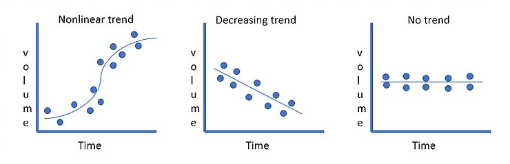
1. Trend component
- The measurement can be taken every hour, day, week, month, or a year or any other regular interval
- The random movements or higher/lower fluctuations over time is called “Trend”
- Example sales volume trend
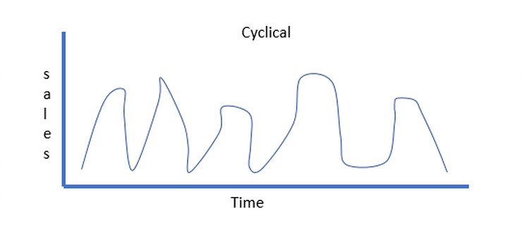
2. Cyclical component
- A cyclic pattern exists when data exhibit rises and falls that are not of a fixed period
- The observations are above or below the trend line
- Example time series for housing cost
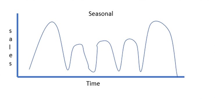
3. Seasonal component
- Seasonality refers to periodic fluctuations.
- For example, sales increase on Diwali.
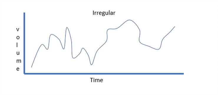
4. Irregular component
- Random variability in data shows the irregular component
- The irregular component is caused by the short term, unanticipated and non-recurring factors that affect the time series
- As it shows random variability in time series, it is unpredictable.
What is stationarity?
It is the most important characteristic of the time series. A time series is said to be stationary if covariance does not change over time that is it has constant mean and variance.
The plot looks something like this,
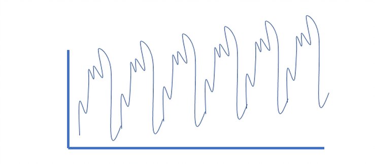
The mean and variance do not vary over time.
Ideally, we want to have a stationary time series for modeling. Of course, not all of them are stationary, but we can make different transformations to make them stationary.
Now let us look at various smoothing techniques to make time-series ready for modeling.
There are many ways to model a time series to make predictions. Here, I will present:
- Moving average
- Exponential smoothing
These techniques are useful for irregular pattern
Moving Averages
It uses an average of most recent n data values in the time series as the forecast for the next period that is the next observation is the mean of all past observations.
Thus, moving average = ∑ (most recent n data values) / n
Let us understand this with an example.
Suppose we have the following data.
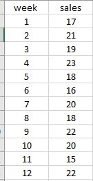
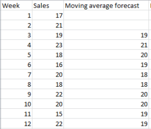
- Now we have to forecast using a moving average, so let’s say we choose moving average = 3.Thus, we have to average the values of the first 3 weeks for week 3. Moving average (weeks 1-3) = 17+21+19/3 = 19 We have to follow the same process for all 12 weeks. Thus, Moving average of all weeks.
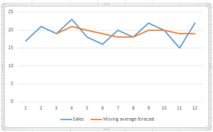
Now let’s plot the actual and forecast graph.
An important consideration in selecting the forecasting method is accuracy. so, let us calculate forecast error and square of forecast error.
Forecast error = actual value – moving average forecast
Squared forecast error= (forecast error)2
Thus, forecast error of week 4 = 23-21= 2
And squared forecast error = 4
Thus, the following table shows the forecast error.
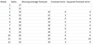
The average of the sum of squared errors is referred to as mean squared error (MSE).
Thus, MSE = ∑ (sum of squared errors) / N = 50/10 = 5
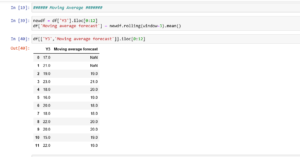
Now let us do a forecast in python
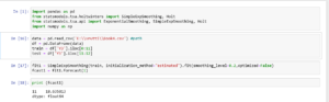
Now let’s use another forecasting method “exponential smoothing”
Exponential smoothing
Exponential smoothing uses a weighted average of past time series values as the forecast. it uses similar logic to moving average, but this time a different decreasing weight is assigned to each observation that is less importance is given to observations moving forward.
Mathematically it is expressed as:
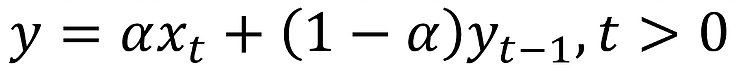
Here,
y = forecast of the time series for period t
Xt= actual value of time series for period t-1
Alpha (a) = smoothing constant between 0 and 1
Yt-1 = forecast of time series for period t-1
Let us take the same example.
Let’s assume alpha value = 0.2.
So for week 3 , Xt = 21 and Yt-1 = 17 (forecast of week2)
So, forecast of week3 = 21*0.2+17*(1-0.2) = 17.8.
Then calculate forecast error for week 3= 19-17.8 =1.2
And squared forecast error for week 3= 1.44
Thus, the following are the final calculations
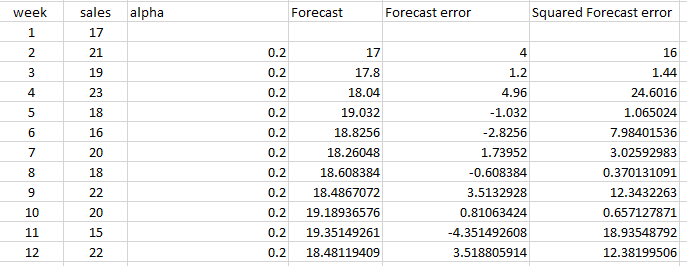
Thus MSE = 98.80/11 = 8.98
Thus, the moving average here is showing low MSE, and it’s better than the exponential smoothing forecast.
Now let us do a forecast in python and check the forecast when sales = 22
Here is the link to my GitHub repo: https://github.com/VruttiTanna/Time-series-forecasting/tree/main
Happy learning 🙂

 11
11
Leave a comment