Optimization is very important for any machine learning algorithm. It is a core component of almost all machine learning algorithms. It is easy to understand and implement. In this article the following topics are covered:
- What is gradient descent
- Intuitive understanding of gradient descent
- How gradient descent works
- Batch gradient descent
- Stochastic gradient descent
- Tips for Gradient Descent
What is gradient descent?
Gradient descent is an optimization technique that finds the values of coefficients of function (f) and minimizes the cost function. It finds the best parameter/coefficient when it is not possible to solve the problem analytically.
Intuitive understanding of gradient descent
Just imagine you are taking part in treasure hunt competition and the treasure is exactly in the bottom of a hemisphere shaped pool. In order to win treasure, you need to dive deep and reach the bottom of pool
Here the pool is the function (f). Any participants who move randomly and try to find treasure on the surface of the water will never win the competition and the participant who dives deep and reach the bottom is the winner.
So participants who are moving randomly are the cost of the current value of coefficients. And the winner is at the bottom which has the best set of coefficients (minimum of function)
So here the goal is to reach a “winning point” that is to evaluate coefficients until they reach “lower” cost.
Thus in machine learning algorithms, we need to repeat this process that will lead you to the bottom of the hemisphere object and have the best values of coefficients at minimum cost.
It looks something like this.
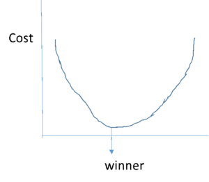
Gradient descent starts by assigning 0 or any small random number for initial values of the function.
Thus coefficient = 0.0
The loss function is calculated by computing the errors of all training samples. Thus derivative of cost is calculated to find the slope of the function so that we know the direction to move the coefficient values in order to get lower cost on the next iteration. For example Actual value is 1 and predicted value is 0 so loss/error/derivative = Predicted – Actual = 0-1 = -1
So if we go back to our example of finding treasure from the pool, the derivative will take us to the bottom of the pool where the treasure lies that is derivative will take us to find minimum loss in algorithm and make us win.
A Cost function basically tells us ‘how good’ our model is at making predictions for a given value of slope and intercept.
Let’s say, there are a total of ’N’ points in the dataset and for all those ’N’ data points we want to minimize the error/loss. So the Cost function would be the total squared error i.e
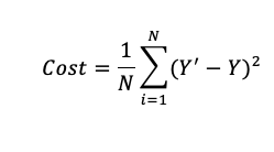
The squared difference makes it easier to derive a regression line. To find the regression line we need to compute the first derivative of the Cost function, and it is much harder to compute the derivative of absolute values than squared values. Also, the squared differences increase the error distance, thus, making the bad predictions more pronounced than the good ones.
Now, we also need to determine the size of steps to be taken to reach the minimum point (that is bottom in our example to reach treasure point), this size of steps taken to reach the minimum or bottom is called Learning Rate. We can cover more area with larger steps/higher learning rate but are at the risk of overshooting the minima. On the other hand, small steps/smaller learning rates will consume a lot of time to reach the lowest point that is we might miss/skip treasure point if we take large steps and if we take small steps then it will consume more time to reach the goal. The learning rate is between 0 and 1.0 and a traditional default value for the learning rate is 0.1 or 0.01, and this may represent a good starting point on your problem.
Thus, the goal of any Machine learning algorithm is to minimize cost function with optimum learning rate to lower error between actual and predicted values gives the best slope and coefficient values, which signifies that the job is well done.
Batch gradient descent
The goal of all supervised machine learning algorithms is to best estimate a target function (f) that maps input data (X) onto output variables (Y ). This describes all classification and regression problems. The different algorithm has different coefficients and its goal is to optimize coefficients that can result in the best estimate of the target function. Common examples of supervised machine learning algorithms are linear regression and logistic regression.
The evaluation of how close a fit a machine learning model estimates the target function can be calculated in a number of different ways, often specific to the machine learning algorithm. The cost function involves evaluating the coefficients in the machine learning model by calculating a prediction for each training instance in the dataset and comparing the predictions to the actual output values then calculating a sum or average error (such as the Sum of Squared Residuals or SSR in the case of linear regression). From the cost function, a derivative can be calculated for each coefficient so that it can be updated using exactly the update equation described above. The cost is calculated for a machine learning algorithm over the entire training dataset for each iteration of the gradient descent algorithm. One iteration of the algorithm is called one batch and this form of gradient descent is referred to as batch gradient descent. Batch gradient descent is the most common form of gradient descent described in machine learning.
Stochastic Gradient Descent
The difference between batch and stochastic gradient descent is, it updates coefficients at each training data point, and thus processing could be slow if we work on large data sets.
The update procedure for the coefficients is the same as that above, except the cost is not summed or averaged over all training patterns, but instead calculated for one training pattern. The learning can be much faster with stochastic gradient descent for very large training datasets and often you only need a small number of passes through the dataset to reach a good or good enough set of coefficients, e.g. 1-to-10 passes through the dataset.
Tips for Gradient descent
- Plot Cost versus Time: Collect and plot the cost values calculated by the algorithm each iteration. The expectation for a well-performing gradient descent run is a decrease in cost each iteration. If it does not decrease, try reducing your learning rate.
- Learning Rate: The learning rate value is a small real value such as 0.1, 0.001, or 0.0001. Try different values for your problem and see which works best.
- Rescale Inputs: The algorithm will reach the minimum cost faster if the shape of the cost function is not skewed and distorted. You can achieve this by rescaling all of the input variables (X) to the same range, such as between 0 and 1.
- Few Passes: Stochastic gradient descent often does not need more than 1-to-10 passes through the training dataset to converge on good or good enough coefficients.
- Plot Mean Cost: The updates for each training dataset instance can result in a noisy plot of cost over time when using stochastic gradient descent. Taking the average over 10, 100, or 1000 updates can give you a better idea of the learning trend for the algorithm.
Conclusion
- Optimization is the big part of any machine learning algorithm and gradient descent is the easiest and simple optimization technique.
- Batch gradient descent refers to calculating the derivative from all training data before calculating an update.
- Stochastic gradient descent refers to calculating the derivative from each training data instance and calculating the update immediately.

 8
8