In this blog I start with understanding of term distribution, then we cover Normal Distribution , its characteristics and some examples.
Distribution : In a simple way term “distribution means” what are the possible values of a variable and what is probability of getting each of these values.
Say we have a piggy bank full of coins , suppose these are 40 coins of 1Re, 30 coins of Rs 2 , 20 coins of Rs 5, 10 coins of Rs 10.
If we draw a coin , it can be either denomination of 1 or 2 or 5 or 10.
Probability of drawing Re 1 coin = 40/100, similarly probability of drawing Rs 2 coin = 30/100,
that of Rs 5 is 20/100 and of 10 is 10/100.
What is it that we try to infer from a distribution ?
A distribution is a way to understand how the data points are clustered or spread across their range of values.
How does a Normal Distribution look like?
Normal distribution, popularly known as bell curve, it is dense in the middle. 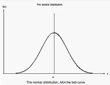
On X axis it has different values variable can take and Y axis has probability.
Majority of data points cluster around the mean, the more away we go from mean the less probability of data point will be.
Geek letter mu represents ‘mean’ value of data points .
Normal distribution is symmetric around the mean 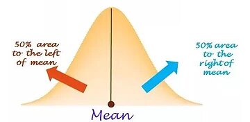
Being symmetric, 50% of data points are below mean and 50% of data points are above the mean.
What parameters are needed for a Normal Distribution?
Normal distribution is determined by parameters (mu) µ and σ (sigma).
µ (mu ) : is population mean , i.e average value of data points
σ (sigma) : is population standard deviation.
The height i.e Y axis , is represented by equation as given here , 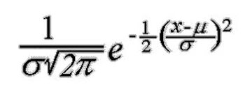
x is data point,
mu and sigma parameters.
68-95-99.7 Rule
- 68% of the population will lie within 1 s.d , 1σ, of the mean
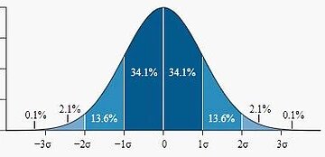
- 95% of the population will lie within 2 s.d , 2σ, of the mean
- 99.7% of the population will lie within 3 s.d , 3σ, of the mean
Lets say average price of paintings of a famous painter is 80,000$ with standard deviation of 20,000$, and underlying distribution is normal.
80,000 + 1 * 20,000 = 100,000
80,000 – 1 * 20,000 = 60, 000
So, there is a 68% chance painting of the famous painter will sell in range of 60,000 to 100,000.
80,000 + 2 *20,000 = 80,000 + 40,000 = 120,000
80,000 – 2 * 20,000 = 80,000 – 40,000 = 40,000
95% chances of selling painting in range of 40,000 to 120,000.
How likely is it to sell painting atleast at 150,000 ?
Z = (150,000 – 80,000)/ 20,000 = 70,000/20,000 = 3.5
Since price of painting is more than 3 sd of average price (which covers 99.7% prices) , so it would be very rare to sell painting at 150,000.
Problem:
Say 2% of produced items are defective with s.d of 0.5% , examine about 5 defects out of 100.
Z = (5-2)/.5 = 3/.5 = 6
Since 6 sd is very far away from mean , so it would be very very rare to see 5 defects out of 100.

 1
1