Logistic regression is one of the most popular machine learning algorithms for binary classification.
For example, we need to classify whether email is spam or not, we need to classify whether medicine will be effective or not etc.
Logistic regression can also help when we want to classify for more than 2 categories that is multinomial logistic regression. For example, classify food into veg, non-veg and vegan.
In this post you are going to discover the logistic regression algorithm for binary classification, step-by-step. After reading this post you will know:
- How to calculate the logistic function.
- How to learn the coefficients for a logistic regression model using stochastic gradient descent.
- How to make predictions using a logistic regression model.
Logistic Binary classification separates data through hyperplane. Logistic regression focuses on maximizing the probability of the data. The farther the data lies from the separating hyperplane (on the correct side), the happier LR is.
The below is the graph.
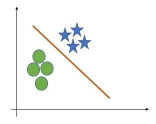
For a binary classification problem, target is (0 or 1).
Before we dive into logistic regression equation, lets take a look at logistic function or sigmoid function, the heart of logistic regression technique.
Logistic function is defined as:
transformed = 1 / (1 + e^-x)
e here is ‘exponential function’ the value is 2.71828
The hypothesis for Linear regression is h(X) = θ0+θ1*X. Therefore, transformed = 1 / (1 + e^-( θ0+θ1*X))
This function squashes the value (any value) and gives the value between 0 and 1.
The sigmoid/logistic function is “S” curve shaped.
Let us take some values on X and then transform it.
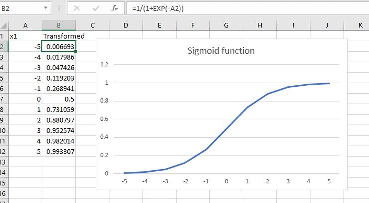
As you can see that we calculated transformed X and then calculated sigmoid function and you can see values between 0 and 1. You can also see that 0 transformed to 0.5 or the midpoint of the new range.
Thus, if probability is > 0.5 we can take the output as a prediction for the default class (class 0), otherwise the prediction is for the other class (class 1).
Let us understand this with a dataset.
The following is a dataset with 3 variables, where X1 and X2 are independent variable and Y is a dependent variable.
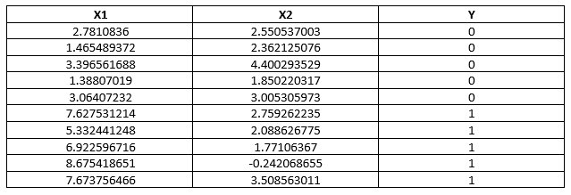
For this dataset, the logistic regression has three coefficients just like linear regression, for example:
output = b0 + b1*x1 + b2*x2
The job of the learning algorithm will be to discover the best values for the coefficients (b0, b1 and b2) based on the training data.
Unlike linear regression, the output is transformed into a probability using the logistic function:
p(class=0) = 1 / (1 + e^(-output))
In your spreadsheet this would be written as:
p(class=0) = 1 / (1 + EXP(-output))
So, logistic regression model has following three steps.
- First, we calculate the Logit function that is h(X) = θ0+θ1*X
- We apply the above Sigmoid function (Logistic function) to logit that is 1 / (1 + e^-( θ0+θ1*X))
- we calculate the error, Cost function (Maximum Log-Likelihood).
So, let us understand error, cost function.
An error in simple terms is (Predicted – actual)
so, if predicted = 1 and actual= 1 then error = 0
so, if predicted = 1 and actual= 0 then error = 1
so, if predicted = 0 and actual= 1 then error = 1
so, if predicted = 0 and actual= 0 then error = 0
If actual y =1 and predicted =0 the cost goes to infinity and If actual y =1 and predicted =1 the cost goes to minimum.
If actual y =0 and predicted =1 the cost goes to infinity and If actual y =0 and predicted =0 the cost goes to minimum.
Logistic regression by Stochastic Gradient Descent
Stochastic Gradient Descent can be used by many machine learning algorithms. It works by using the model to calculate a prediction for each instance in training set and calculate error for each prediction.
We can calculate coefficients for logistic regression model as follows:
Given each training instance:
- Calculate a prediction using the current values of the coefficients.
- Calculate new coefficient values based on the error in the prediction.
This process is repeated until the model is accurate enough for fix number of iterations.
Calculate prediction
Let us initialize all coefficients with 0 and calculate probability of first training instance that belongs to class 0 that is X1 = 2.7810836, x2=2.550537003, Y=0.
B0 = 0
B1 = 0
B2 = 0
prediction = 1 / (1 + e^ (-(b0 + b1*x1 + b2*x2)))
prediction = 1 / (1 + e^ (-(0.0 + 0.0*2.7810836 + 0.0*2.550537003)))
prediction = 0.5
Calculate New Coefficients
b = b + alpha * (y – prediction) * prediction * (1 – prediction) * x
Alpha is learning rate and must be specified at beginning. It controls, how much the coefficient changes each time and usually its between 0.1 and 0.3, here we will take 0.3
Here, B0 (intercept) will not have x value so it is assumed as 1 every time.
Let’s update the coefficients using the prediction (0.5) and coefficient values (0.0)
b0 = 0 + 0.3 * (0 – 0.5) * 0.5 * (1 – 0.5) * 1.0 = -0.0375
b1 = 0 + 0.3 * (0 – 0.5) * 0.5 * (1 – 0.5) * 2.7810836 = -0.104290635
b2 = 0 + 0.3 * (0 – 0.5) * 0.5 * (1 – 0.5) * 2.550537003 = -0.09564513761
Now, repeat this process for X1 = 1.465489372, x2= 2.362125076, Y=0.
b0 = -0.0375
b1 = -0.104290635
b2 = -0.09564513761
prediction = 1 / (1 + e^ (-(-0.0375+ 0.0*-0.104290635+ 0.0*-0.09564513761)))
prediction = 0.397
Let’s update the coefficients using the prediction (0.397) and coefficient values
b0 = -0.0375 + 0.3 * (0 – 0.397) * 0.397* (1 – 0.397) * 1.0 = -0.06605
b1 = -0.104290635+ 0.3 * (0 – 0.397) * 0.397* (1 – 0.397) * 1.465489372= -0.1461
b2 = -0.09564513761+ 0.3 * (0 – 0.397) * 0.397* (1 – 0.397) * 2.362125076= -0.1631
so, we have to repeat this until last data point that is for all 10 samples and learning on all samples for one time is called one epoch.
Thus, the first epoch coefficients are as follows:
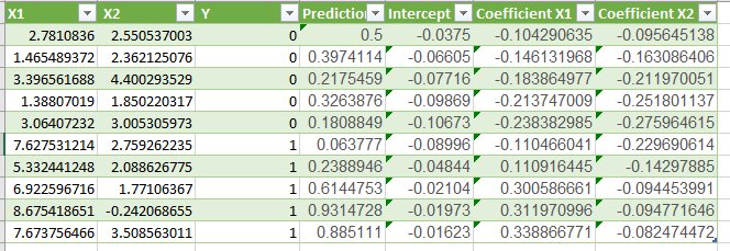
b0 = -0.01623
b1 = 0.3388
b2 = -0.0824
We are repeating it for 10 times and thus 10th epoch is as follows:
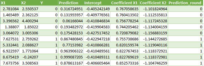
Thus, final coefficients are:
b0 = -0.4066054641
b1 = 0.8525733164
b2 = -1.104746259
As you can see the last column “prediction_round” that is if prediction is < 0.5 then 0 else 1.
So, accuracy is:
accuracy = (correct predictions / number predictions made) * 100
accuracy = (10 /10) * 100
accuracy = 100%
Thus, you can now take new data and get prediction value.
Summary:
In this post we covered how to implement logistic regression from scratch step by step and we covered:
- Calculating logistic function
- Calculate coefficients using stochastic gradient descent.
- Make predictions using logistic regression
you can share your comments and put your questions in discussion forum
here is the link :
https://www.datascienceprophet.com/forum
Happy learning 😊

 6
6